Harvest Imaging Blog

From the measurements of the row FPN and the column FPN, it was learned that the device-under-test (DUT) has a large shading component in dark.  (Shading refers to a gradual change of a particular parameter from top to bottom and/or from left to right.)  So it will be a very valuable exercise to measure this shading component.

To evaluate the dark shading, the same images are used as before : multiple dark images taken at room temperature and at different integration times.  To quantify the dark shading, the images taken at an exposure time of 8 seconds are used : at 8 seconds, the average dark signal is about 25 % of the saturation level.  Because dark shading is the low frequency variation of the dark signal, the following procedure is followed :

–       all images captured at 8 seconds integration time are averaged, in this way the temporal noise will be reduced,

–       the averaged image will be forced through a low-pass filter with a 9×9 filter kernel.  This operation will reduce the (high-frequency) FPN.

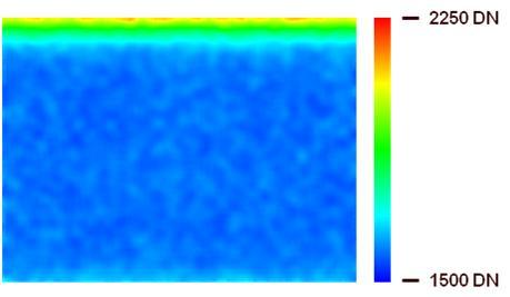
The result after averaging and filtering is shown in figure 1.

 Figure 1 : low-frequency variation in dark signal at 8 second integration time.

Clearly visible in figure 1 is the non-uniformity of the dark signal.  Its value is slightly increasing towards the lower side of the sensor, but it is strongly increasing towards the top side of the sensor.  From left to right the dark signal seems to be more constant.  This result is in full agreement with the column FPN and row FPN calculated in an earlier blog.  Those results indicated already a large variation in average row value, while the average column value was nearly constant.

The shading illustrated in figure 1 can be expressed as :

–       the peak to peak value, equal to 561 DN,

–       maximum-minimum value, equal to 2116 DN and 1555 DN respectively.

In principle these numbers are more or less meaningless without any further “reference”.  The additional parameters needed are :

–       evaluation temperature, being room temperature,

–       integration time, being 8 seconds,

–       dark signal offset, being 819 DN,

–       average dark signal in dark without offset correction, being 1637 DN,

–       average dark signal in dark with offset correction, being 818 DN.

Comparing these numbers one can state that the dark signal shading is pretty large compared to the average signal in dark.  This can have some very annoying consequences : dark reference lines/columns are always located next to the active pixels.  So these references lines and columns can be situated in part of the sensor where the dark signal is deviating quite a bit from the average dark signal and/or the average dark signal in the center part of the sensor.  In this way the dark reference signal generated by the signal processing will be too high, and image details in dark might get lost ! 

In the case of such a large dark shading with possible issues with the dark reference lines, another way of creating a black reference is needed :

–       or using black reference columns with the risk of generating row-wise noise,

–       or using a black reference frame and perform a dark compensation on pixel level.

Success !

Albert, 23-11-2011.

This week CEI organized another session of my Hands-On Characterization course in Dresden.  A new group of enthousiastic engineers registered for the course.  As could be expected the course is improving time after time.  The feedback from the participants again was very positive, and that is a strong encouragement to continue in the same direction.  This means further improvement of the course where necessary, and adding new measurement assignments to the course.  New and additional equipment is already ordered to keep the course up to date !

Almost all of the participants succeeded in finding/measuring/calculating the conversion gain of the test-camera.  Personally I do see this as the highlight of the course.  That so many participants came to right value is a remarkable success, because it is not a really simple measurement to do.  Making a Photon-Transfer Curve (PTC) seems to be fairly simple if you have some experience, but can be difficult if you have to do this for the first time.  But once the participants have the knowledge of how to create a PTC, other measurements become simple as well.  In many cases it is a matter of calculating averages and calculating standard deviations.  It is just a matter of doing this things in the right order !

At this moment my Hands-On Characterization course is only organized by CEI.  And up to now CEI is using 4 different course location : Barcelona, Copenhagen, Dresden and Cambridge.  Unfortunately the transport of the equipment needed in the course is not so easy.  Transporting by a courier is tricky because the equipment is pretty vulnerable, and tranporting by car (as I did up to now) takes a lot of time.  For that reason CEI will organize the next Hands-On Characterization course in Amsterdam (in May 2012).  This is much closer to my home, which makes the transport of the equipment much easier.  Moreover, Amsterdam is also very easy to reach from all over Europe, making the travelling for the participants very smooth as well.  Looking forward to see some of my readers in Amsterdam 😉

Albert, 16-11-2011.

Column FPN was the subject of the previous blog, so it will not be any surprise that this time the row FPN will be discussed.  To calculate (!) the row FPN in dark, the same data or images as before are being used.  The following procedure is followed :

–       After removing/correcting the defect pixels, all images taken at a particular exposure time are averaged on pixel level, resulting in one (average) image per exposure time,

–       Next, per row all pixels are being averaged, yielding an average value for every row (at every value of the exposure time),

–       Once the row averages are available, the standard deviation on these average row values is calculated.  In principle a single number will be found for all measurements done at every exposure time.

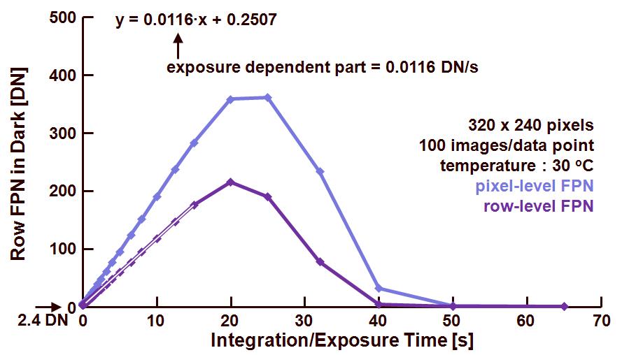
The result of this calculation is shown in figure 1, indicating the row FPN in dark as a function of exposure time.

 Figure 1 : row fixed-pattern noise in dark as a function of the exposure time.

There are two curves shown :

–       the first represents the pixel-level FPN, already discussed in a previous blog,

–       the second one is showing the row FPN in dark, which is only a bit lower than the pixel FPN.  The following data can be obtained from the curve : 2.4 DN is the row FPN at 0 s exposure time, and the time depending part of the row FPN equals to 0.0116 DN/s.  At 25 % of saturation level or an exposure time of 8s, the row FPN is equal to 93 DN rms.  Taking into account the absolute values mentioned earlier, the row FPN can be calculated to be equal to 5.7 % at 25 % of saturation.

The ratio between the DSNU on pixel level and the row FPN is equal to : 0.0188/0.0116 = 1.6, whereas the theoretical value would predict : (number of columns)^0.5 = 17.9.  To find out where this large discrepancy (more than a factor of 10 !) is coming from, the uniformity of the average row value of every row is checked at a particular exposure time (8 s).  The result is shown in Figure 2.

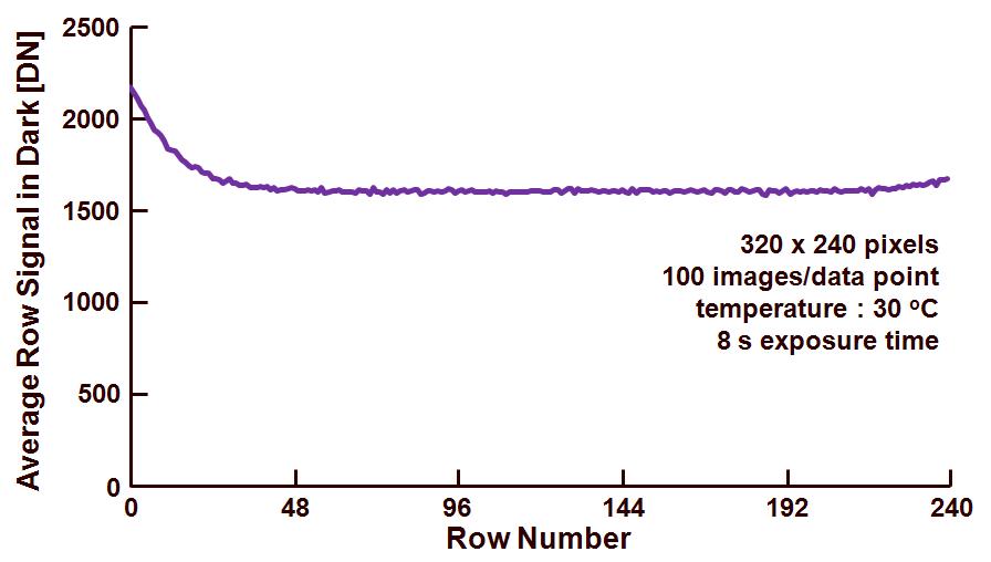
 Figure 2 : average row signal in dark at 8 s exposure time.

As can be learned from the data in Figure 2, the average row value is absolutely not constant (also expressed by the high row FPN rms value).  The figure clearly shows a large shading component in the average dark signal.  This is the origin of the large row FPN and the fact that the ratio of pixel FPN over the row FPN does not follow the theoretical value. 

Of course the large value for the row FPN is indicating a large non-uniformity of the average dark values on row level.  But the origin of this non-uniformity does not necessarily need to be found in the row circuitry, the origin is coming from somewhere else.  That will be the subject of next blog.

Albert, 01-11-2011.