In the meantime there should be enough explanation about the slanted edge method in this blog, it is time now to do the measurements. For those of you who want to get quick results with the slanted edge method, you can follow the rules/guidelines/advices of the ISO-12233 standard, buy the testchart, install the software, and get going. Of course, it is much more fun to develop the whole stuff yourself, and by the way, that is the proper way to learn all the details about the slanted edge method for the MTF characterization.
So now the first measurement results of the slanted edge method will be highlighted. The various steps to come to the appropriate results go as follows :
- Focus an object/target with a slanted edge (preferably between 2o and 10o) on the imager,
- Grab 50 images of the slanted edge object and average these images to lower the temporal noise,
- Grab 50 images of a uniform target (without changing the camera settings, without changing the light source) and average these images to lower the temporal noise,
- Grab 50 images in dark (without changing the camera settings) and average these images to lower the temporal noise,
- Correct the slanted image data for non-uniformities in dark and for non-uniformities in pixel response and/or non-uniformities of the light source,
- Select a smaller window of the image in which the slanted edge is present,
- Calculate the slope of the slanted edge w.r.t. the vertical column or horizontal row direction of the imager, the slope of the slanted edge is needed to calibrate/normalize the horizontal spatial frequency axis of the MTF curve,
- Record the spatial frequency response (SFR) in 4 adjacent columns, merge the 4 SFR’s and perform a further data interpolation, to get equidistant data point in the spatial domain,
- Calculate the line-spread function (LSF) based on the 4-times oversampled SFR,
- Force the LSF through a fast-Fourier transform, resulting in the optical transfer function and calculate the magnitude of the latter to obtain the modulation transfer function,
- Normalize both axes to get the classical MTF curve.
Figure 1 shows some intermediate steps of the MTF characterization. The left part of figure 1 illustrates the observed slanted edge, in a window of 100H x 350V pixels. The slanted edge is created by means of the edge of a MacBeth chart in front of a white sheet of paper. The middle part of figure 1 shows a randomly chosen horizontal line (in red) along which the dark-light transition is checked. Through this dark-light transition the pixels values along a vertical column (in green) are used for the SFR measurement. Finally, the right part of figure 1 shows the calculated slanted edge (in blue).
Figure 1 : Three illustrations of the observed slanted edge : left the raw data coming off the sensor, middle : row and column along which the SFR is measured, right : the slanted edge as calculated by the software tool.
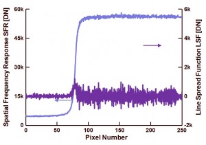
Figure 2 shows the SFR and LSF based on the pixels values shown in figure 1 and after 4 times oversampling of the data (= using the data of 4 adjacent columns).
Figure 2 : Spatial Frequency Response after 4x oversampling.
As can be seen by means of the SFR on figure 2, the transition from dark (left side) to light (right side) is relatively steep, but this steepness is much less visible in the LSF in figure 2. The latter has to do with the 4x oversampling, which reduces the difference between two neighbouring measurement points. Also remarkable is the relative large variation in the white background used in the measurement. But these variations show up at a relative high frequency and will not influence the MTF measurement.
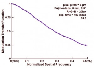
The final MTF result is show in Figure 3.
Figure 3 : MTF obtained by the slanted edge method.
The measurment with white light (R=G=B) results in an MTF of 0.25 or 25 % at Nyquist frequency. For a pixel with a large fill factor (the exact value is not known, but the pixel pitch is large and with micro-lenses, a large fill factor can be expected) this number of 0.25 or 25 % is relatively low. It should be noted that not just the sensor MTF is measured, but the measurement does include the camera lens as well !
Albert, 06-10-2014.


Albert,
congratulations first for your recent SEMI award.
concerning the slanted edge:
there is a plugin box for ImageJ.
SE_MTF_2xNyquist.jar
Easy to use, it worked in some way,
but i did not like the final results competely at the end.
regards
heinrich
Need to emphasize that the SFR is measured along the horizontal line, and not along the vertical line.
You are right, good catch !
Thanks for reminding me.
Albert.
Hi Albert,
Can you please help me with a few questions:
1. The pixel value we collect from dark to light, are they refer to as ESF or SFR…? It looks like SFR (from Figure 2’s description), but I think in some of your earlier blogs they are called ESF?
2. If Figure 2 is using the data of 4 adjacent columns in Figure 1, that means the data of 4 adjacent green vertical lines in Figure 1, correct? But then the dark-light transition is checked by the red horizontal line…I’m quite confused about the function of each line, can you help to clearify a bit?
3. What is the calculated slanted edge in the right part of figure 1 used for? To get the slope of the slanted edge so we can calibrate/normalize the horizontal spatial frequency axis of the MTF curve? Can you help to explain this a little more?
Thanks for the awesome article!
1. You are right, it is called SFR. (Spatial Frequency Response)
2. You are right, again. The horizontal red line is just an indication where you do the evaluation of the MTF. MTF can be dependent on the location in the image. Mostly the center part has a higher MTF than the corners of the image. Do not pay too much attention to the red line. Just an indication, nothing more, nothing less.
3. The blue line across the slanted edge only indicates that the software tool to measure/calculate the MTF has (automatically) found the right edge. Also here, just an indication, nothing more, nothing less.
Albert.
Thanks for the explanation, Albert!
hello, there’s a statement “preferably between 2 and 10 degrees.” is there any reason? Thanks
Yes, there is a reason, you should not come too close to perfect alignment with the columns (or rows), that is the reason to chose a value larger than 2 degrees. To avoid any errors, you should stay below 10 degrees (unless you oversample and re-interpolate).
Albert.