Over the last few years a lot of information about the Photon Transfer Curve (PTC) is being published in this blog. The influence of many different sensor parameters on the PTC was studied and described. For those of you that are still hungry to get more information, please remember that Jim Janesick wrote a complete book about the PTC. It was Jim who developed this wonderful technique in the ‘80s for CCDs, but the PTC is perfectly applicable to CMOS imagers as well. The great advantage of this measuring method is the fact that no absolute measurements of any light input is needed.
In this blog, the application of the PTC on the data/images collected earlier will be described. So the same images (with light on the sensor) as used in the previous blogs are being re-used. What was done to generate these images : the sensor under test was uniformly exposed to light, while varying the exposure time. For every exposure time applied, several images were grabbed, the average value of the obtained images as well as the temporal noise on pixel level was calculated.
The measured signal of the sensor can be written as :
Stot = kNo + Soff (1)
While the measured temporal noise on pixel level can be written as :
stot2 = k2sR2 + k2so2 (2)
with :
– Stot : measured output signal [DN],
– k : conversion gain [DN/e–],
– No : number of optically generated electrons,
– Soff : offset signal [DN],
– stot : total temporal noise measured [DN],
– sR : temporal noise associated with the readout channel [e–], also the noise floor in dark at 0 s exposure time,
– so : photon shot noise [e–].
And with :
so2 = No = (Stot – Soff)/k (3)
the total noise can be written as :
stot2 = k2sR2 + k(Stot – Soff). (4)
The signal-to-noise ratio of the system under consideration can be written as :
Stot/stot = (Stot-Soff)/( k2sR2 + k(Stot – Soff))0.5. (5)
The obtained measurement data/images can be used to create :
1) Standard deviation versus average effective signal, both on a log-scale (“Mean-Standard Deviation”).
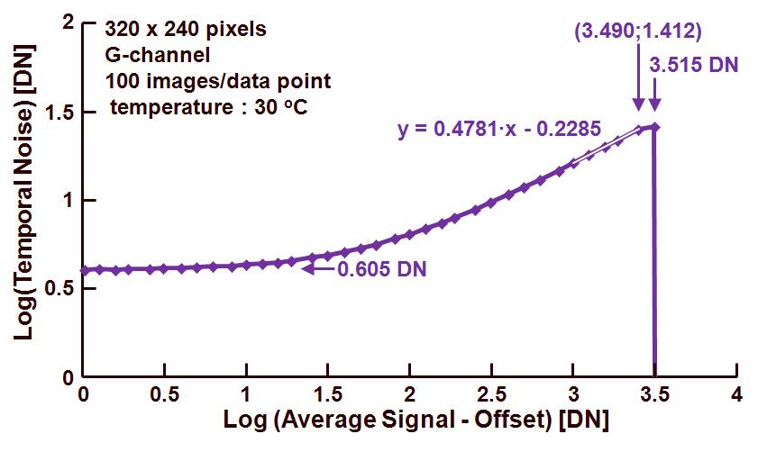
The standard deviation is representing the temporal noise of the pixels, the effective signal is equal to the average output signal minus the DC-offset of the output signal. The obtained curve is shown in Figure 1.

Figure 1. Photon Transfer Curve : standard deviation versus effective output signal.
From left to right, one can recognize three parts in this PTC graph :
– A flat part in which the temporal noise of the readout channel or the noise floor at 0 s exposure time, is dominant, in the example shown this noise is equal to 100.605 DN = 4.03 DN. This can also be derived from equation (4) and scrapping the photon shot noise :
stot2 = k2sR2 or stot = ksR.
– A part with increasing noise for increasing effective signal, in this region the photon shot noise is dominant, and the slope of the curve needs to be equal to 0.5 (or at least very close to this value). The regression line drawn through this part of the curve is characterized by the relation shown in the graph. Using equation (4) again, but this time focusing on the photon shot noise, it reduces to :
stot2 = k(Stot – Soff) or k = 1/(Stot – Soff) at stot = 1 DN.
In this way the conversion gain k can be found by extrapolation of the regression line towards the crossing with the horizontal axis. The value found for k is : 10-(0.2285/0.4781) = 0.33 DN/e–. Be aware that this method actually requires the curve to get a slope = 0.5 before any extrapolation can be done. In this example the slope is only 0.4781. Although this value is pretty close to 0.5, a substantial error can be introduced into the calculation of the conversion factor. For that reason a better method to find the conversion factor is in the “Mean-Variance” technique, explained further in this blog.
– The part at which the noise reaches a maximum value and for any further increase in effective signal, the curve collapses. This is the point at which the pixels reach their saturation level. In the example shown, this happens for an effective output signal equal to 103.515 DN = 3273.0 DN.
2) Variance versus average effective signal, both on a linear scale (“Mean-Variance”).
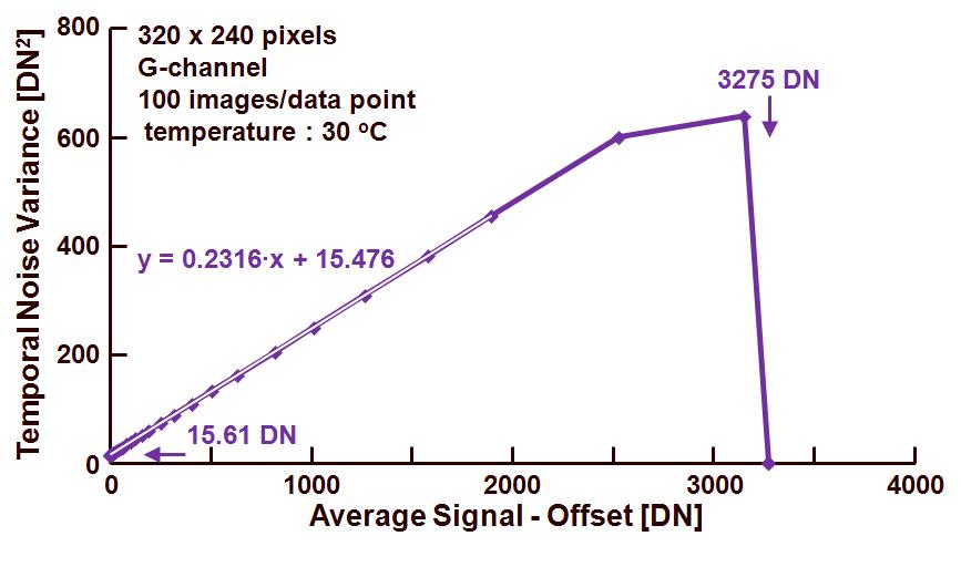
The curve obtained is illustrated in Figure 2.

Figure 2. Photon Transfer Curve : noise variance versus effective output signal.
Also this figure shows some interesting features from left to right :
– Crossing with the vertical axes (= 0 DN effective signal) for a noise variance equal to 15.61 DN. This value corresponds to the temporal noise at very low signal values or noise floor in dark for 0 s exposure time, and actually should represent the variance of the noise associated with the readout channel. The value found here is 15.610.5 DN = 3.95 DN.
– A linear part in the curve for which the relation is shown in the figure. In this region again formula (4) is valid :
stot2 = k2sR2 + k(Stot – Soff).
Taking into account the relationship of the regression line, it should be concluded that the conversion gain k (being the slope of the line) is equal to 0.23 DN/e–. This value is lower than the one previously found with the Mean-Standard Deviation method. This is due to the fact that there is a relative large error introduced in the calculation because the slope of the noise versus signal curve is not perfectly equal to 0.5 !
– A saturation part with a collapsing curve for a maximum signal level of 3275 DN, being the saturation level of the pixels.
3) Signal-to-noise ratio versus average effective signal, both on a log-scale (“Mean-Signal-to-Noise”).
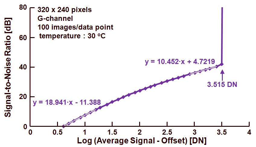
The relation between signal-to-noise ration and effective signal is shown in Figure 3.
 Figure 3. Photon Transfer Curve : signal-to-noise ratio versus effective output signal.
A similar story as before can be repeated about three different regions in the curve :
– At the very left end a first part that can be linearized is indicated by the relation between signal-to-noise and average effective signal. In this region the noise of the readout channel is dominant, and based on equation (5), the signal-to-noise ratio can be written as :
Stot/stot = (Stot-Soff)/(ksR) or ksR=Stot-Soff at Stot/stot = 1.
In this example, the readout noise is equal to 1011.388/18.941 = 3.99 DN.
– Just before saturation, a second linear part can be recognized in the region where the photon shot noise is the dominant noise source, and based on equation (5), the signal-to-noise ratio can be simplified to :
Stot/stot = ((Stot-Soff)/k)0.5 or k = 1/(Stot-Soff) at Stot/stot = 1.
In this example, the conversion gain is equal to 104.7219/10.452 = 0.35 DN/e–. Also this value deviates from the previously calculated values, because the extrapolation of the data can introduce some nasty errors.
– Finally the signal-to-noise ratio is becoming extremely large, due to the fact that the temporal noise of the sensor is reduced to almost zero at saturation of the pixels for a value of 103.515 DN = 3273 DN.
In conclusion, parameters such as the readout noise or noise floor in dark, the conversion gain and the saturation level can be found by means of the Photon Transfer Curve. But the most accurate and reliable data for (although 3 different curves are used, the input data for these curves is the same) :
– the conversion gain can be obtained via the Mean-Variance curve,
– the readout noise or noise floor in dark at 0 s exposure time, can be obtained via the Mean-Standard Deviation curve,
– the saturation level can be obtained by any form of PTC.
The PTC curve can be constructed in various ways. In this blog uniform illuminated sensor areas at various exposure times are used, in the next blog a few alternatives will be highlighted.
Albert, 27-08-2012.
Hi Albert,
First thank you so much for posting the “How to Measure” series, I learned a lot from this. I hope I can also attend one of those “hands on” workshops in US also.
I have a question about the total temporal noise. I took a look of Jim Janesick’s PTC book. I found that in his book, the total noise includes read noise, shot noise and FPN noise. But here based on the equation, the total temporal noise seems don’t contain FPN noise. In Janesick’s book, he use “total noise” for “Mean-standard deviation” plot and “temporal noise variance” for “mean-variance” plot. So in your case, why the total noise doesn’t have FPN component? And how do you calculate the total temporal noise from captured images? Is it calculated as the squre root of variance of all the pixels?
Thanks,
Dengyu
Hi, very good question !
I do calculate the temporal noise of EACH pixel by calculating the standard deviation of all values of ONE particular pixel in multiple frames. If you take only the values of ONE pixel into account you avoid the FPN, because you do not include the content of neighbouring pixels. This method can be repeated for every pixel of the image.
Success, Albert.
Hi Albert,
Thanks for your quick response. So if I want to calculate the temporal noise for the whole image sensor area. Can I calculate the standard deviation along multiple frames for each pixel, and then average the whole area?
Another question is that I found in Janesick’s book, for the “mean-standard deviation” method, the total noise includes FPN noise, but for the “mean-variance” method, the noise is just temporal noise. However, in your descriptions, both methods seems like have the same temporal noise, is it different from Janesick’s description?
Best,
Dengyu
On your first question, the answer is bascially YES, but please not that averaging multiple noise values is statistically not correct. I suggest to take the median value of all calculated noise values.
In my descriptions, I Always calculate the noise along multiple frames for each pixel. In this way I can avoid any FPN in my calculation. The FPN calculation/measurement is another characterization.
Albert.
Hi Albert,
Thanks for the reply. So does it mean that in your “Mean-standard deviation” curve, there is no “FPN regime” as shown in Janesick’s PTC plot, i.e., the regime with slope=1? Since you avoid FPN in your calculation? Just want to double check:-)
Best,
Dengyu
Dengyu, as I mentioned, if you work on pixel level across multiple images, the FPN is not taken into account and you will not find the slope=1 part of the curve. Albert.
Hi Albert, thank you so much for the information. I really appreciate that. That clarifies my thought.
Hello Albert,
I get a PTC using the first approach, in log scale and slope is around 0.3. What could explain that? and using the second method there are many kinks in the plot rather than a straight line.
Regards,
Arvin
Hi Arvin,
The answer is very simple : “I do not know”. This is the same situation as if you call your medical doctor to tell him/her that you have some pain in your finger. Then what will your doctor tell you ? Most probalby he/she will ask you to come to visit him/her so that he/she can diagnose the situation. Without seeing anything I cannot tell you what the origin could be. Can you tell me how you did the capturing of the images ? DC light source !? Fixed gain !? Did you correct for the offset of the signal !?
If you prefer, you can contact me off-line.
Regards, Albert.
Hi Albert,
Thanks for quick reply.
It would be great if we can discuss off-line.
Regards,
Arvin
Hi Albert,
Could only one photo diode measure PTC ?
The noise term of PTC comes from std of photo diode array.
If only one photo diode, how to calculate noise term for PTC using ?
Thanks.
Ataru
I still enjoy this tutorial very much, even after nine years.
There is still room for improvement, though. The units and annotations in Figure 1 are in a slight mismatch with regards to the explanatory text below it.
Example: Noisefloor is labeled “0.605 DN” in the plot, but 10^0.605 DN in the text. Same goes for the saturation level (3.515 vs 10^3.515)
The reason for this confusion of course it the log axis, and with it the whole “one cannot take the logarithm of a unit, should normalize, etc. etc.”
I would suggest to normalize both x and y by DN (i.e. log(Temporal Noise / DN) [abs.]) and use unitless numbers in the plot instead of an ambiguous “DN”.
Or just leave it as it is, no plot is perfect 😉
Hi Christian, thanks for your valuable comment. If I can find the time, I will update the material, but the main issue is time …
Albert.
Hi,
I just want to confirm which of these is the correct/best calculation approach to get the y-axis values for plotting (across ONE pixel at ONE integration time for simplicity):
1. Average across many frames to get mean signal (for the pixel) and then sqrt(mean signal – offset) -> Poisson mean/variance/standard deviation relationship of shot noise
OR
2. Perform a basic standard deviation formula (summation formula) for that set of frames
Also, correct me if I am wrong but I believe the shot noise in this case includes dark signal shot noise too as it should increase by the same Poisson relationship, with time.
Cheers
Hello, You item 1) is the one that I most frequently use. This gives the best results up to now.
And yes, you are right, when taking measurements with light, the pixels also contain dark current. To minimze the latter, try to use enough light power so that the light signal overrules the dark current signal.
Success, Albert.
Thank you for you swift reply!
That does, however, leave me with a bit more confusion:
If you are using Poisson statistics to calculate the pixel values before you plot them (STDEV = SQRT(MEAN) for Poisson because VAR = MEAN for Poisson) this should technically result in a Mean-Variance plot that has a slope of 1 because Mean = Variance in Poisson.
In other words, in your reply you mentioned that you get the standard deviation for a pixel by doing SQRT(mean-offset) and then plot the values, as per poisson statistics. But this would suggest that your Mean-Variance curve should have Y values corresponding to same X value magnitude because SQRT(mean-offset)^2 = mean-offset -> the same as on the X axis. However, your Figure 2 graph has a slope of 0.2316 so I can only assume that I am misunderstanding something in your calculations.
Apologies for the long reply.
Thank you again!
For the PTC curve, you plot on the X-axis the log(signal-offset) and on the Y-axis the log(temporal noise) which is equal to log(standard deviation).
For the mean variance curve, you plot on the X-as the signal-offset (linear scale) and on the Y-axis the variance of the noise. If you do both parameters in the charge domain, you are right, you will find a slope of 1. If you do both parameters in the voltage or digital domain, you will find the conversion gain.
BE AWARE : variance = mean value if ONLY valid in the charge domain, not in the voltage or digital domain !!!
Albert.