After several months of silence, here is a new blog about measuring image sensors. This time the blooming and/or anti-blooming of an imager is analyzed. Actually in this first blog about blooming, it will be shown how NOT to measure blooming.
Blooming is the effect that is showing up in the case of strong overexposure of the image sensor. If the pixels are seen as a buckets and the photon-generated electrons are seen as the water contained in these buckets, it is clear that the maximum amount of water that can be stored in the bucket is limited. If more light is falling on the pixels, more water needs to be stored in the buckets. But once a bucket is completely filled, any extra water is going to spill over to the neighbouring buckets. The last effect is being known as blooming. Any means in the pixel to prevent blooming is called anti-blooming.
The intention of the measurement reported in this blog, is to check out the anti-blooming capabilities of an image sensor. Ideally this can be done by overexposing a single pixel and check any blooming in the neightbouring pixels, but that is not easy to realize. An alternative way of measuring the anti-blooming capabilities is to use a colour sensor and illuminate the device with monochrome light. If the sensor is illuminated with blue light, the green and red pixels will have a smaller light sensitivity to blue light and the blue pixel will saturate much faster than the green and red pixels. Once the blue pixel is saturated, its anti-blooming should become active. Without anti-blooming, the blue pixel will spill over its charge into the green pixel (direct neighbours) and red pixel (diagonal neighbour). If spilling occurs, the sensitivity of the green and/or red pixel will increase and this can be measured by monitoring the green and red output signal.
What is explained above is realized and the result is shown in Figure 1.
 Figure 1 : Response of the different colour planes (R, G, B) of a CMOS sensor under illumination with blue light (470 nm).
For the three colour planes, the regression line of the linear response is created as well. The ratio between B and G response is 4347/1119 = 3.9. The ratio between B and R response is 4347/140 = 31. Unfortunately (for the measurement), no change in response can be seen in the G or R channel once the B channel is saturated. Conclusion the anti-blooming towards direct neighbours is at least a factor 3.9, towards diagonal neighbours is at least a factor 31.
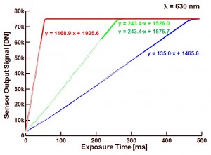
A similar measurement can be done with red light. The result is illustrated in Figure 2.
 Figure 2 : Response of the different colour planes (R, G, B) of a CMOS sensor under illumination with red light (630 nm).
This time, the ratio between R and G response is 1169/243 = 4.8. The ratio between R and B response is 1169/135 = 8.7. Unfortunately (for the measurement), no change in response can be seen in the G or B channel once the R channel is saturated. Conclusion the anti-blooming towards direct neighbours is at least a factor 4.8, towards diagonal neighbours is at least a factor 8.7.
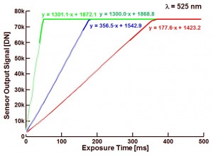
Finally, the sensor was illuminated with green light, and the 3 colour channels were checked as shown in Figure 3.
 Figure 3 : Response of the different colour planes (R, G, B) of a CMOS sensor under illumination with green light (525 nm).
The ratio between G and B response is 1301/365 = 3.6, the ratio between G and R response is 1301/178 = 7.3. Also for this situation no blooming artifacts can be found.
In conclusion : the anti-blooming capabilities are at least for direct neighbours a factor of 7.3, for diagonal neighbours a factor of 31. These numbers are relatively small, but the measurement technique applied is not capable of doing better. The numbers reported are limited by the characterization method and not by the sensor. So actually, what is shown in this blog is how NOT to measure the anti-blooming of a sensor, unless your device-under-test has a very poor anti-blooming performance.
Albert, 10-08-2015.
Thanks for the post. I am excited to see more updates on this topic 🙂
Thanks for publishing this series of posts. Still reading …
To me, in figure 2 there actually seems to be a change in sensitivity of blue and green, after red has saturated. The regression line of blue crosses the plot two times. I bet when you split the regression line and leave some space between both of them, there’ll be a difference in slope.
I know it does not matter. Reading on …
Thomas, thanks for the comment.
I do think that the effect you mention is more a measurement/sensor/camera inaccuracy than a blooming effect. Normally blooming occurs first towards direct neighbouring pixels. For figure 2 this would mean from red pixels into green pixels. And the green pixel is reacting pretty linear, even after the red pixel is saturated. On the other hand, the blue pixel is a diagonal neighbour of the red pixel, and blooming is much more unlikely. Even if your suggestion is applied to split the regression line into two parts, you will see that the second part of the regression line gets a smaller slope, but actually with blooming, you would expect a steeper slope.
I do hope that this explanation is clear to you. Otherwise let me know. Albert.