After measuring the noise in dark on pixel level, it is important to check the noise in dark on column level and on row level. This time we will discuss the temporal noise on column level. The latter can be calculated based on the same data/images used for the FPN in dark and used for the noise in dark on pixel level. It is just a matter of applying the right order of statistical calculations. To evaluate the noise in dark on column level, all pixels in each column are averaged and next the rms value is calculate on these average column values. Once the noise for each column is known, the average of all rms values is calculated.
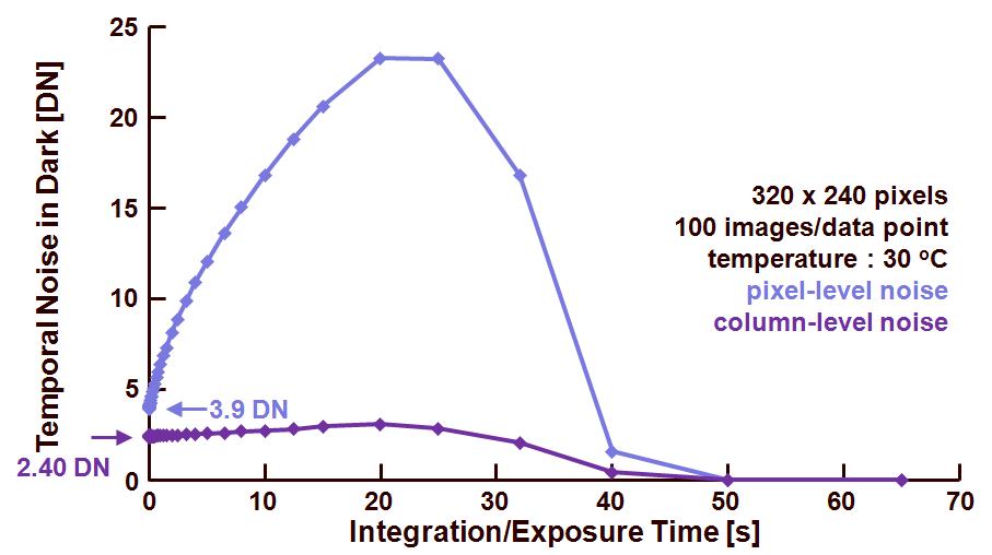
The result of this process is shown in Figure 1. Both the temporal noise on pixel level (previous blog) and the temporal noise on column level are shown as a function of integration time.

Figure 1. Temporal noise measured in dark on pixel level and on column level, as a function of the exposure or integration time.
As can be expected, the column level noise is much lower than the pixel level noise, although the difference between the two curves is minimum at 0 s exposure time and at saturation. At lower exposure times, the temporal noise of the electronic circuitry plays the most important role, and because the difference between pixel and column noise is not that much, it can be expected that most of the total temporal noise in dark is coming from the column circuitry. For larger values of the exposure time, the dark shot noise is dominant and in that case, the averaging effect on the data removes this pixelized noise component. At saturation, the noise is reaching its minimum value.
Numbers that are obtained :
– At 0 s exposure time, the temporal noise on column level is 2.40 DN,
– At 25 % of saturation, and for an exposure time of 8 s, the temporal noise on column level is 2.66 DN.

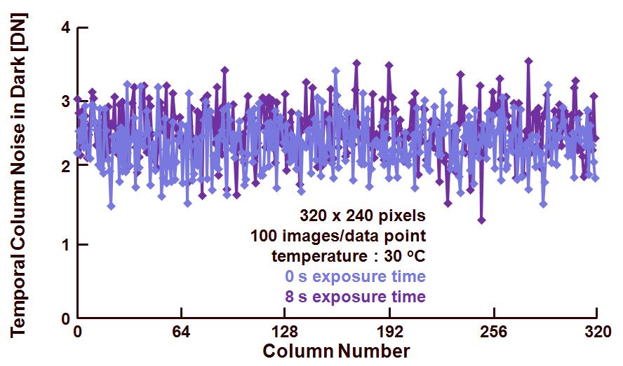
Figure 2. Column noise in dark for two different integration times.
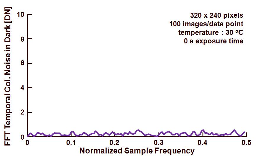
Figure 2 shows the column noise in dark for two integration times : 0 s (to get the noise without any dark shot noise) and at 8s (when the pixels containing 25 % of the full well capacity). In both cases no repetitive pattern in the noise can be recognized, this is also verified by means of a FFT calculation. The result of this is shown in Figure 3.

Figure 3. FFT of the signal of the column noise calculated for an exposure time of 0 s.
As can be observed in Figure 3, there is no specific FFT signal available at a particular frequency. From this, one can conclude that the column noise is randomly distributed.
Next time a similar exercise will be done for the temporal noise in dark on row level.
Albert, 27-06-2012.